Chapter 9 Basic Plotting

R is particularly powerful in plotting graphs and figures. The generic function to use is plot() which gives you a graphical view of the relationship between your data points.

> plot(1:10)

The plot() function takes many default arguments. One of the most important arguments is the way your data is to be plotted: you either indicate type='l' for lines, or type='p' for points or type='b' for both of them. As seen above, the default is p.

> plot(1:10, type='b')

There are many more arguments that you can use to change the appearance of your plot. Let’s look at a few of them using the following two example vectors:

> x <- seq(1, 100, length.out=20)
> y <- log(x) + (x/100)^5

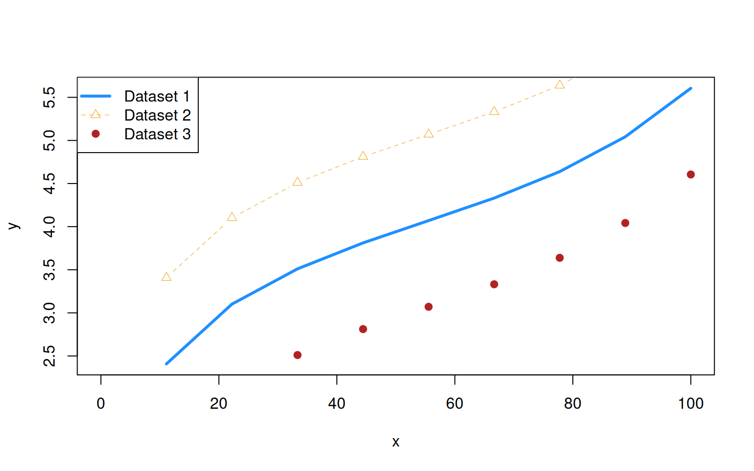
The first things that you usually want to do is to give your plot a title and to properly annotate the axis. The former is achieved with the argument main, the latter with the arguments xlab and ylab that label the x-axis and y-axis, respectively. The default axis labels are the names of your variables, and they are often not very informative.

> plot(x, y, xlab='X axis', ylab='Y axis', main='A nice plot')

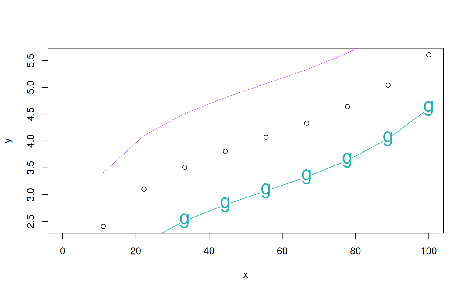
The following arguments are used to change the appearance of the plotted data:

• col defines the color. You can either provide the name of a built-in color (you can get all available colors using the function colors()), or the numbers 1-8 that are matched to basic colors.
• pch defines plotting characters. The numbers 0-25 indicate different symbols, but you can also use any character.
• cex (for character expansion) defines the size of your plotting characters. Default is cex=1 and larger values increase the size of the plotting character.
• lwd defines the line-width, i.e. how think lines are to be drawn. The default is lwd=1.
• lty defines the line type. you can either provide a number between 0-6, with 0 being blank (i.e. no line), 1 solid, 2 dashed and so forth, or a combination of two characters from 1, 2, …, 9, A, …, F to indicate the length of dashes and spaces. lty=1F, for instance, would result in very short dashes with lots of space between them.

Here is an example of how to use these options.

> plot(x, y, type='b', col="mediumvioletred", pch=5, cex=2, lwd=0.5, lty=3)

Importantly, all these options can also provided as vectors with one element per data point. If the vectors are shorter, they get recycled.

> randomColors <- colors()[sample(1:length(colors()), size=length(x))];
> plot(x, y, col=randomColors, pch=3:12)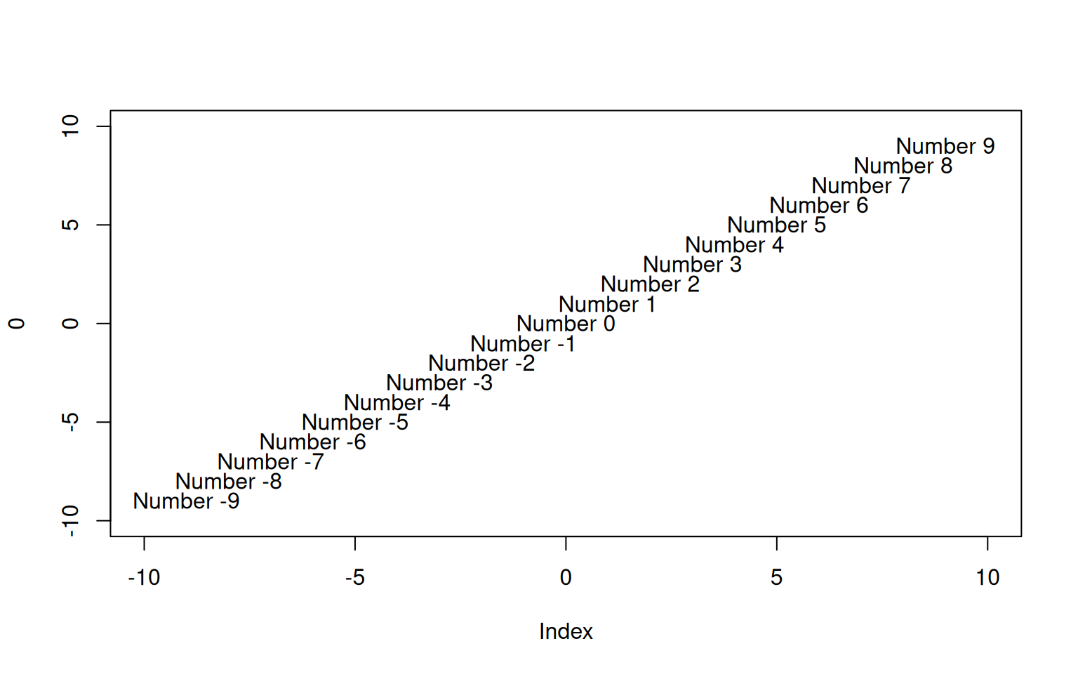

Generally, if you don’t know how to plot something, the ?plot help function is a good place to start, and a quick google search get you usually even faster to a solution.

9.0.1 Permanent Changes: the par() function

Setting graphics parameters with the par() function changes the value of the parameters permanently, in the sense that all future calls to graphics functions will be affected by the new value. The par() function allows also to set additional graphical parameters including mar to set the margins.

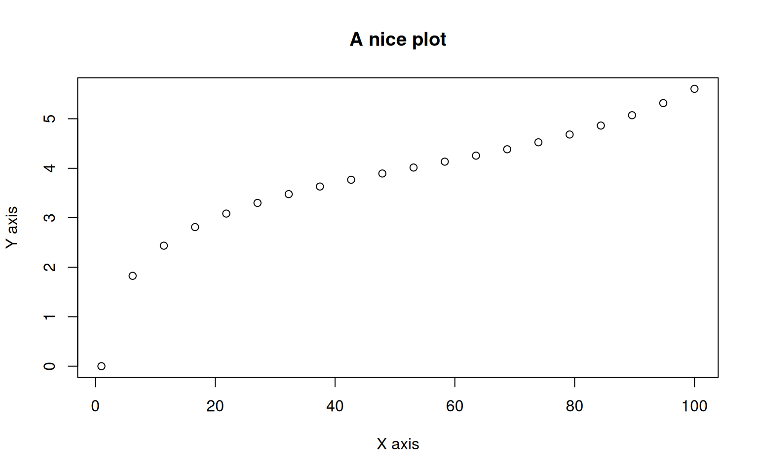
> x <- 10*(0:10)
> y <- log(x) + (x/100)^5
> par(mar=c(4,4,0.1,0.1), lty=2, pch=19)
> plot(x,y, type='b', xlab="The variable x")

If you check ?par you will see that the list of options is close to endless and allows to specify pretty much any aspect of your plot.

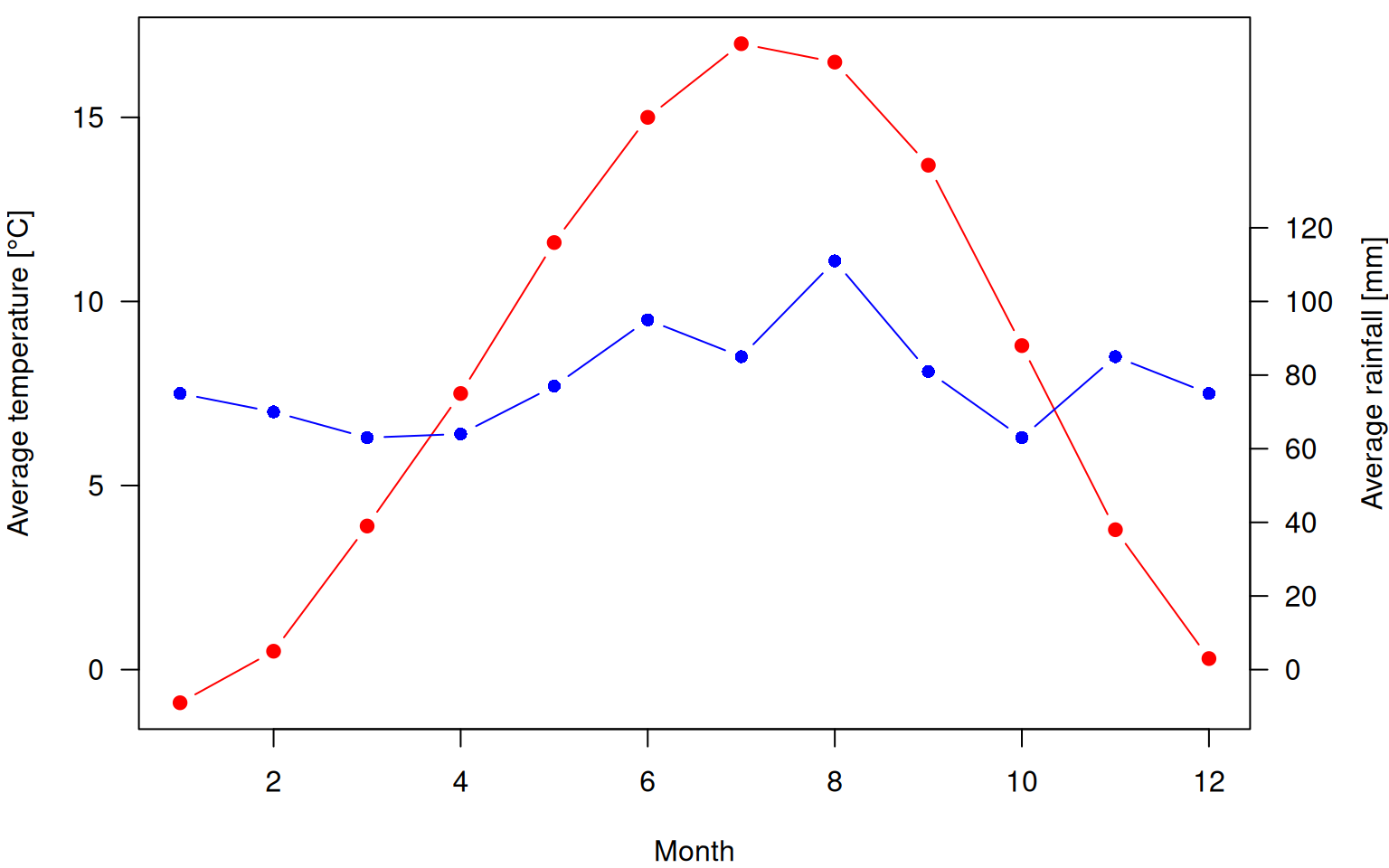
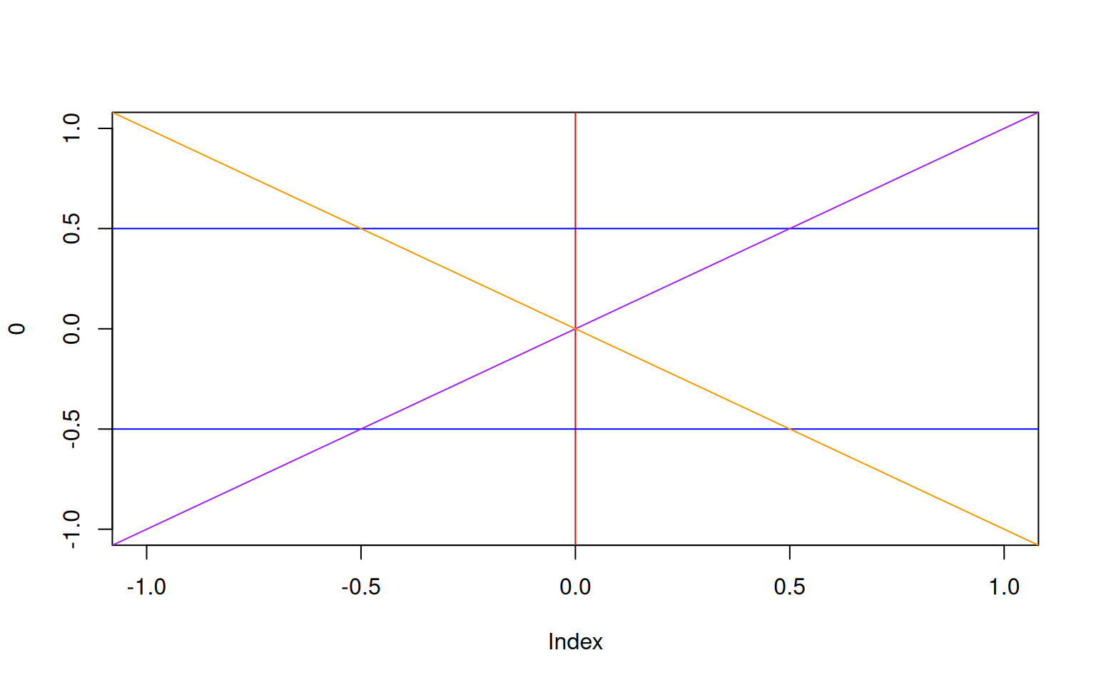
In addition to specifiying grapical parameters, the par() function can also be used to retrieve current settings by providing the name of the graphical parameter of interest. par("lty") for instance returns the current line type set. In many cases the call par("usr") is particularly useful as it returns a vector of length 4 specifying the coordinate system of the plot: the first pair of values give the x-values at the left-most and right-most position, respectively, and the second pair gives the y-values of the bottom and top of the plot.

> plot(1, xlim=c(-2,2), ylim=c(-1,1))

> par("usr")
[1] -2.16  2.16 -1.08  1.08

As the above example illustrates, R adds some extra space by default. This behavior, while mostly useful, is easily turned off using xaxs='i' and yaxs='i' for the x and y axis, respectively.

> plot(1, xlim=c(-2,2), ylim=c(-1,1), xaxs='i', yaxs='i')

> par("usr")
[1] -2  2 -1  1

9.0.2 Exercises: Basic Plotting

See Section 18.0.21 for solutions.

1. Create a vector x of length 20 with equally spaced values between -5 and 5. Then, create a vector y with elements $y_i=2x_i^2$. Plot y against x using red filled circles connected by dashes. Label the axis “My variable x” and “Some transformation of x” and give the plot the title “The plot of a noob”.

2. Plot y against x again, but this time as a solid, thick line. Use a random color, add no title nor axis-labels and modify the margins to maximizes the area used for the plot itself.

3. In R there are length(colors()) predefined colors. Make a plot with a grid of 26x26 points, colored by following the list of available colors. Use large squares as symbols.

4. Plot the numbers 1-100 as filled circles and color them in red if they are a multiple of 7 and in orange other wise.