Chapter 10 Probability Distributions

As a statistical language, it is no surprise that R comes with many tools for working with probability distributions, as well as implementations of most standard distributions. In this chapter, we will introduce these tools, focusing first on the most general of all distributions: the normal or Gaussian distribution.

10.0.1 The normal distribution

The normal distribution is defined through the density function

$f (x | μ, σ^{2}) = \frac{1}{\sqrt{2 π} σ} e^{- \frac{(x - μ)^{2}}{2 σ^{2}}}$ ,

where $μ$ denotes the mean (first moment) and $σ^{2}$ the variance (second moment). If $μ = 0$ and $σ^{2} = 1$ , the resulting distribution is termed the standard normal distribution, usually denoted by $φ (x)$ .

Let’s first use R to have a look at this density function. For this, we will use the function dnorm() that returns the density of the standard normal distribution at any point.

> x <- seq(-4, 4, length.out=100)
> plot(x, dnorm(x), ylab="density")

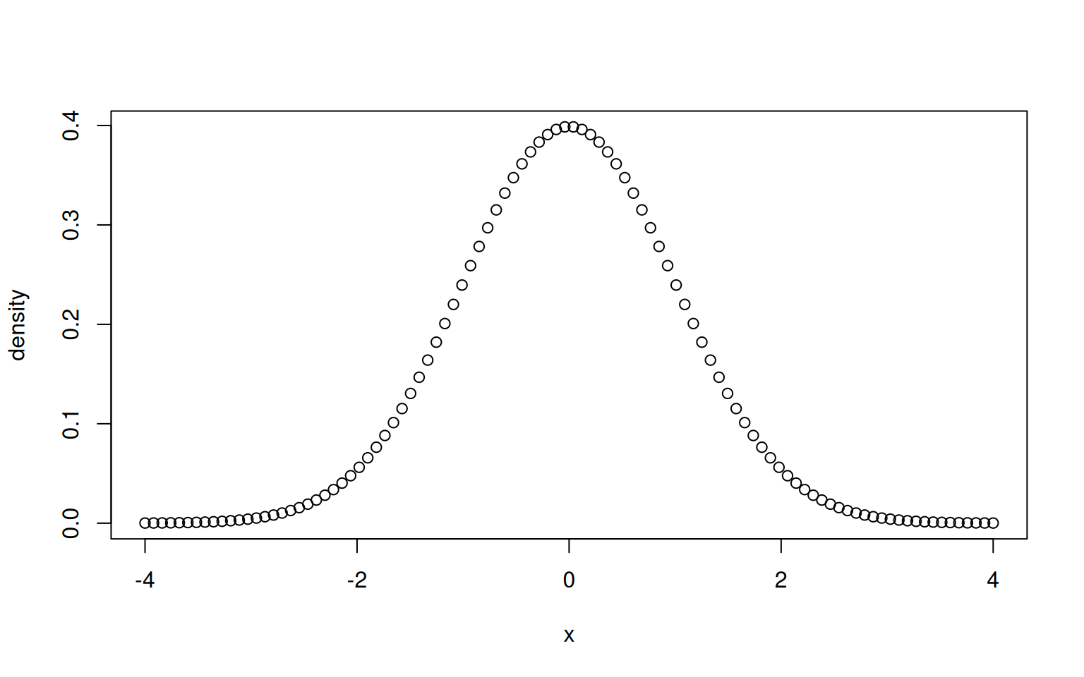
The function dnorm() can also be provided the meanand sd of the normal distribution, that is, the mean $μ$ and the standard deviation $σ = \sqrt{σ^{2}}$ .

> plot(x, dnorm(x), ylab="density", type='l')
> lines(x, dnorm(x, mean=1), col='red')
> lines(x, dnorm(x, mean=-1, sd=2), col='blue')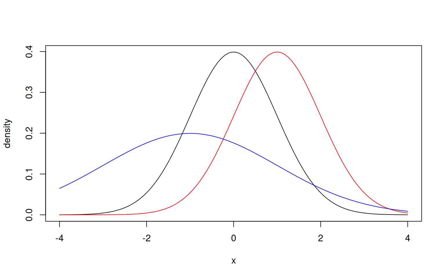

In addition to the density function, R provides three equally important functions for the normal distribution:

The cumulative distribution function (CDF) $F (x | μ, σ^{2}) = \int_{- \infty}^{x} f (x | μ, σ^{2}) d x$ , which is the integral of the probability density function from minus infinity up to $x$ . The corresponding R function is pnorm().
The quantile function $Q (q | μ, σ^{2}) = F^{- 1} (q | μ, σ^{2})$ that, given a quantile $q$ , specifies the value of $x$ such that $F (x) = q$ . The corresponding R function is qnorm().
A function to generate random samples from the normal distribution: rnorm().

The cumulative distribution function gives us important information about the location of a value within the distribution, also called quantile, with 0 implying the far left and 1 the far right. Specifically, it gives us $F (x | μ, σ^{2}) = P (X \leq x | μ, σ^{2})$ which is the probability that a random value from the distribution $X$ is smaller or equal to $x$ .

To illustrate this, let’s plot the quantiles:

> plot(x, pnorm(x), ylab="CDF", type='l')
> lines(x, pnorm(x, mean=1), col='red')
> lines(x, pnorm(x, mean=-1, sd=2), col='blue')
> abline(h = 0.5, lty = 2)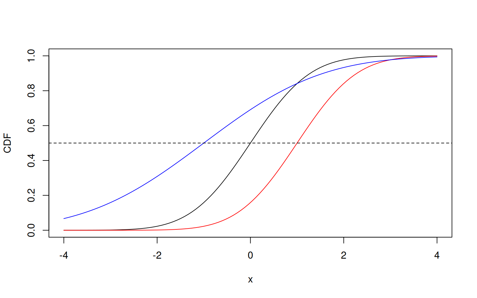

We see that the cumulative distribution function is monotonically increasing within the interval [0,1]. This means that for infinitely small values of $x$ , the CDF is zero: $lim_{x \to - \infty} F (x) = 0$ ; and for infinitely large values of $x$ , the CDF is one: $lim_{x \to \infty} F (x) = 1$ . All other values of $x$ will hence be somewhere in between zero and one.

In addition, since a normal distribution is symmetric around the mean, $F (μ | μ, σ^{2}) = \frac{1}{2}$ in all cases. This is visible in the plot, where the dashed line crosses the curves exactly at their mean.

> pnorm(0)
[1] 0.5
> pnorm(1, mean=1)
[1] 0.5
> pnorm(-2, mean=-2, sd=10)
[1] 0.5

However, values far away from the mean have quantiles that are either close to zero or one.

> pnorm(1)
[1] 0.8413447
> pnorm(1, mean=5)
[1] 3.167124e-05

By definition, the quantile function qnorm() is the inverse of the cumulative function:

> x <- 2
> q <- pnorm(x)
> qnorm(q) == x
[1] TRUE

We can use qnorm() to answer the question: What is the value of $x$ for the $p^{t h}$ quantile of the normal distribution? For example, what is the value of $x$ for the 50th quantile of the standard normal distribution?

> qnorm(0.5)
[1] 0

The answer is zero, since the mean (= the 50th quantile) of the standard normal distribution is zero. Or, what is the value of $x$ for the 99th quantile of the standard normal distribution?

> qnorm(0.99)
[1] 2.326348

This results in a large value of $x$ , which makes sense since 99% of all random values from the distribution are smaller or equal to $x$ .

We can of course also plot the inverse cumulative distribution function:

> quantiles <- seq(0, 1, by = 0.01)
> plot(quantiles, qnorm(quantiles), ylab="x", type='l')
> lines(quantiles, qnorm(quantiles, mean=1), col='red')
> lines(quantiles, qnorm(quantiles, mean=-1, sd=2), col='blue')
> abline(v = 0.5, lty = 2)

Again, the dashed line at the 50%-quantile intersects the curves exactly at their mean. In fact, this is the same plot as above for pnorm(), except that the x- and y-axis are switched!

The last function rnorm() returns a vector of random numbers from a normal distribution. Its first argument n specifies the length of the random vector returned and is mandatory.

> rnorm(1)
[1] -2.897464
> rnorm(10, mean=100)
 [1] 100.56478  99.25415  97.34809 100.26004 102.59361  99.26100  99.76211
 [8] 100.50752  98.13695 100.05297

Note that since these numbers are drawn at random, your numbers will likely be somewhat different. We will talk more about the issue of randomness below.

10.0.2 Other Distributions

As mentioned above, R implements basically all standard probability distributions using the same syntax:

The probability density function starts with a d followed by an (abbreviated) name referring to the distribution.
The cumulative density function starts with a p followed by an (abbreviated) name referring to the distribution.
The quantile function starts with a q followed by an (abbreviated) name referring to the distribution.
The function to generate random numbers starts with a r followed by an (abbreviated) name referring to the distribution.

Among the many distributions implemented, the following are noteworthy:

The uniform distribution with name unif with parameters minand max.
The Binomial distribution with name binom with parameters size and prob that refer to the number of trials and the probability of a success.
The exponential distribution with name exp and parameter rate (usually written as $λ$ ).
The Poisson distribution with name pois with parameter lambda.
The Beta distribution with name beta with parameters shape1and shape2 (usually written as $α$ and $β$ ).

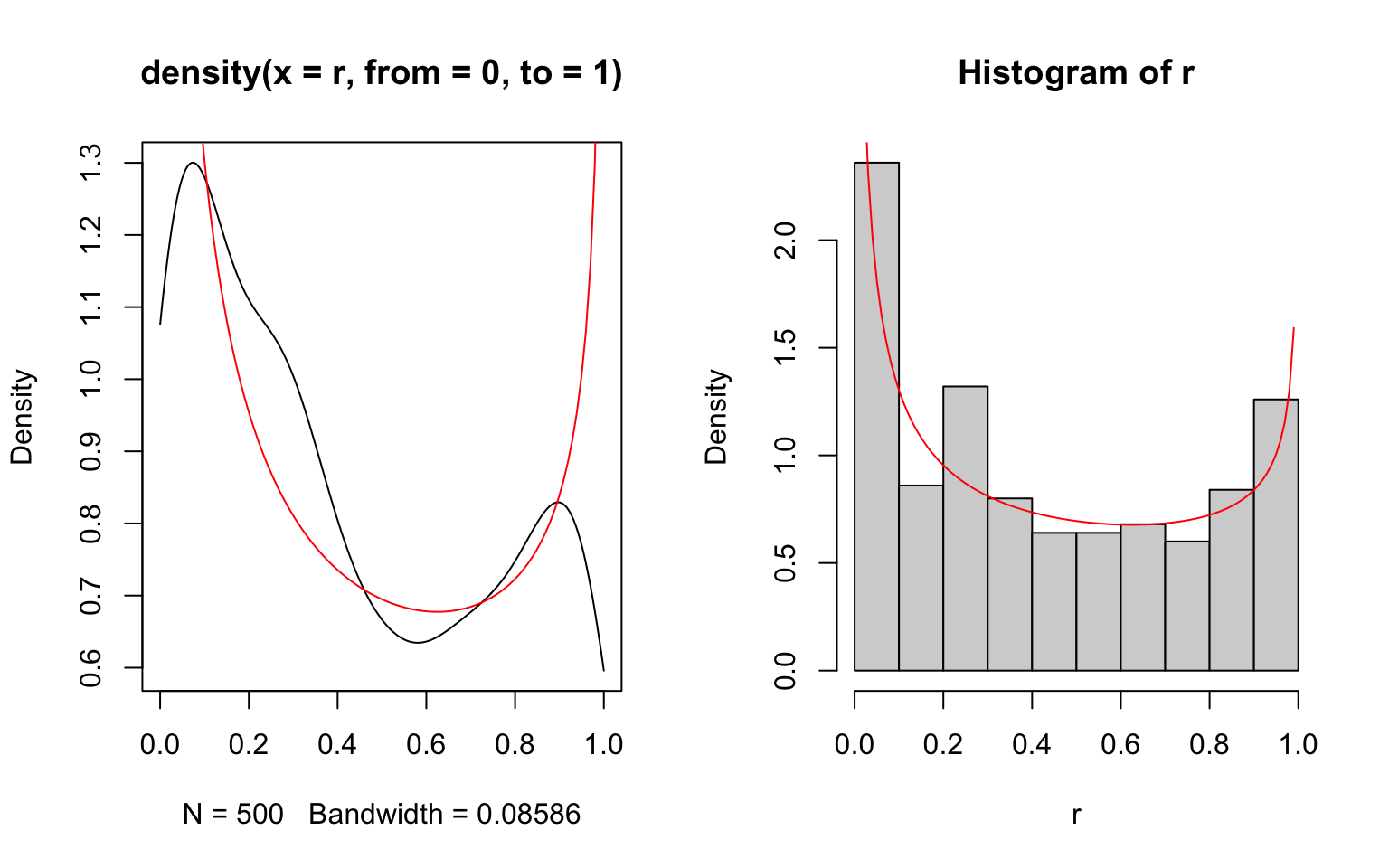
To plot the beta distribution, for instance, we can use

> x <- seq(0, 1, length.out=100)
> plot(x, dbeta(x, 0.5, 0.6), ylab="density")

Note that all distribution functions take vector input. To generate random values from a Poisson distribution with different rates, you may provide a vector of lambdas:

> rpois(10, lambda=seq(1, by=20, length.out=10))
 [1]   0  20  46  61  80  98 100 133 172 176

Sometimes you may want to simulate outcomes according to some fixed probabilities. For instance, you may want to simulate the cases 1,2 and 3 with probabilities 0.1, 0.7 and 0.2, respectively. As we have seen before, this can be achieved with sample()

> x <- sample(1:3, size=1000, prob=c(0.1,0.7,0.2), replace=TRUE)
> sum(x==2) / length(x) # approximately 0.7
[1] 0.702

In case we only have two possible outcomes, we may also use the uniform distribution between 0 and 1. Indeed, the probability that a random value $X < p$ is just $p$ . Hence, a vector of outcomes with probability $p = 0.73$ can be simulated as

> x <- runif(1000) < 0.73
> sum(x) / length(x) # approximately 0.73
[1] 0.732

10.0.3 Setting the Seed

Random numbers have the inherent property to be hardly reproducible. While this is often a desired property, it can be very cumbersome for debugging, since the results change every time we run a script.

To generate random numbers, R uses an algorithm that starts with an initial number (the so-called seed), and then generates consecutive numbers based on this. The seed hence completely defines the sequence of pseudo-random numbers. By default, R uses the current time as a seed. Therefore, when we run e.g. runif() twice, it results in different numbers, since the time and therefore the seed is different:

> runif(5)
[1] 0.64748013 0.05790647 0.15457335 0.56983298 0.32648175
> runif(5)
[1] 0.6516352 0.9364190 0.6460917 0.7883878 0.4038033

However, we can define our own seed with the function set.seed(). It expects a number as an argument that will be used as a seed. What number we use doesn’t matter at all. R creates the same random numbers every time we run the script:

> set.seed(13); runif(5)
[1] 0.71032245 0.24613730 0.38963444 0.09138367 0.96206454
> set.seed(13); runif(5)
[1] 0.71032245 0.24613730 0.38963444 0.09138367 0.96206454

Using a different seed will again create different random numbers:

> set.seed(14); runif(5)
[1] 0.2540337 0.6378273 0.9571886 0.5525467 0.9830671

10.0.4 Exercises: Probability distributions

See Section 18.0.24 for solutions.

What is the probability density of $x = 0.15$ under an exponential distribution with rate $λ = 2$ ?
What is the probability density of $x = 3$ under a Poisson distribution with $λ = 2$ ?
What is the value $x$ such that a random value from a normal distribution with mean $μ = 5$ and variance $σ^{2} = 4$ is smaller than $x$ with a 99% probability?
What is the probability density of $x = 0.72$ under a beta distribution with both shape parameters $α = 0.7$ and $β = 0.7$ ?
What is the value $x$ such that a random value from a standard normal distribution is larger than $x$ with a 30% probability?
Generate 100 random values from a Poisson distribution with $λ = 2$ .
Generate 13 random values from a exponential distribution with rate 0.5.
Simulate $10^{3}$ values from a standard normal distribution. What is the fraction of those values that are < -1? What is the theoretical expectation? Do you get closer to the theoretical expectation with more random draws?
Simulate $10^{3}$ values from a binomial distribution with size 10 and probability 0.1. What is the fraction of those values that are > 2? What is the theoretical expectation?
Human heights are approximately normally distributed, with a mean of 164.7 cm and a standard deviation of 7.1 cm for females and a mean of 178.4 cm and a standard deviation of 7.6 cm for males. Plot the two probability density functions (use heights ranging from 140cm to 200cm). Add a vertical line at your own height to the plot. What is the probability density of your height?
Let’s revisit the normal distributions for human height from the previous exercise. Plot the cumulative distribution function for both male and female heights, using the same parameters as above. Add a line at your own height to the plot. What is the quantile for your own height (i.e. what is the probability to be smaller or equal your height)?
Let’s revisit the normal distributions for human height from the previous exercise. What male or female heights represent the 5%, 32%, 50%, 68% and 95% quantile, respectively? Again plot the probability density functions, and add these heights as vertical lines in order to illustrate the quantiles.
Replicate the two plots regarding the probability density function and the cumulative distribution function on the Wikipedia page for the exponential distribution.
Simulate a random walk as follows:
1. Initialize the random walk with $x_{1} = 0$
2. Sample the next value $x_{t + 1} \sim N (x_{t}, 1)$ from a normal distribution with mean $x_{t}$ of the previous value and variance $= 1$ .
3. Repeat step 2 until you reach $x_{100}$ .
4. Plot the full random walk as purple filled dots connected by lines.
Simulate the Martingale System for betting. In this system, a player bets on a color in a roulette game and thus has a $18 / 37$ chance of winning, in which case the invested money is doubled (if you invest 4 CHF and win, you’ll have 8 CHF). The idea of the martingale system is to start with a modest investment of 1 CHF. Whenever you loose, you double the invest for the next round. As soon as you win, you stop the game. Simulate playing roulette according to this system until the player won or had to invest more than 100 CHF. Do such simulations 1000 times. How often did the player win? What was the average net benefit across replicates?