11.1 Exporting and Importing Data Frames
11.1.1 Exporting
The most generic way to save a data frame is with the function write.table().
This file will look like this:
"ID" "Random"
"1" 1 0.0742941116914153
"2" 2 0.961419784929603
"3" 3 0.447386628715321
Note that by default, write.table() adds the row index as row names (the numbers in quotes at the beginning). This behavior can be modified using the argument row.names that either accepts a vector with alternative row names, or can be set to FALSE to omit row names altogether. This is usually the preferred option.
The resulting file will now look like this:
"ID" "Random"
1 0.0742941116914153
2 0.961419784929603
3 0.447386628715321
Important other optional arguments are:
col.names: works just likerow.namesbut for the columns.append: when set toTRUE, will append the data to an exisiting file rather than overwriting it.sep: specifies the field separator to be used (default is a white space).quote: specifies whether characters and factors should be written in quotes (default isTRUE).
Here is a more complicated example:
> d <- data.frame(Number=c(1,3,5), Animal=c("Lion", "Chimpanzee", "Flamingo"))
> write.table(d, "animals.txt", sep = "\t", row.names=FALSE)
> # append to file
> f <- data.frame(a=c(7,2), b=c("Lynx", "Falcon"))
> write.table(f, "animals.txt", sep = "\t", row.names=FALSE, append=TRUE, col.names=FALSE)
The resulting file will look like this:
"Number"    "Animal"
1   "Lion"
3   "Chimpanzee"
5   "Flamingo"
7   "Lynx"
2   "Falcon"
11.1.2 Importing
A file such as this one can be read back from the file system using the function read.table().
> read.table("animals.txt")
      V1         V2
1 Number     Animal
2      1       Lion
3      3 Chimpanzee
4      5   Flamingo
5      7       Lynx
6      2     Falcon
Note that by default, read.table() does not expect column names and will thus interpret the first row as data. To have the first row properly interpreted as column names, use the argument header and set it to TRUE.
> read.table("animals.txt", header=TRUE)
  Number     Animal
1      1       Lion
2      3 Chimpanzee
3      5   Flamingo
4      7       Lynx
5      2     Falcon
The function read.table() also offer many useful optional arguments:
sep: specifies the field separator to be used (default is a white space).nrows: limit import to the first n rows only.skip: indicates the number of rows to skip before reading. This is helpful for files that have comments at the beginning.stringsAsFactors: whether or not R should convert strings into factors. The default value forstringsAsFactorsdepends on your R version (new versions have defaultFALSE). IfstringsAsFactorsisTRUE, the column Animal is turned into factors:
> read.table("animals.txt", header=TRUE, stringsAsFactors=TRUE)$Animal
[1] Lion       Chimpanzee Flamingo   Lynx       Falcon
Levels: Chimpanzee Falcon Flamingo Lion Lynx
If this is undesired, we may turn this conversion off:
11.1.3 Other input and export options
While write.table() and read.table() are generic functions with many options that can handle all export and import problems, many options have to be tuned in some cases. This is why R offers two sets of functions for specific use cases:
Comma separated values files, so-called CSV files, are a common data exchange format that can be imported and exported by Calc, Excel or other spreadsheet programs. In such files, each line contains one data record with values (columns) separated by a delimiter. In contrast to what the name suggests, most spreadsheet programs actually use a semicolon
;and not a comma,as delimiter. While CSV files can be written and read using the standard functionwrite.table()andread.table(), the functionswrite.csv()andread.csv()orwrite2.csv()andread.csv2()are easier to use as they offer better defaults. The difference between these is that the.csv()functions use commas,and the.csv2()functions use semicolons;as delimiters.Instead of commas or semicolons, many people also use tabs to separate data fields. For such files, the functions
write.delim()andread.delim()offer more useful defaults.
Finally, R also offers the possibility to write files line-by-line using the function cat(). By default, cat() prints to the console.
However, cat() has the optional arguments file and append that can be used to build files.
The above code will create a file “myfile.txt” that looks like this
Hello world!
1 2 3 4 5 6 7 8 9 10
11.1.4 Importing from a URL
The functions introduced above can also read data provided via a URL. For this, the URL has to be turned into a connection using the function url(), and this connection can be provided to any reading function.
As an example, consider the weekly number of deaths happening in Switzerland as provided by Swiss Federal Statistical Office here.
The relevant CSV file can be directly imported into R.
> d <- read.csv2(url("https://www.bfs.admin.ch/bfsstatic/dam/assets/12607335/master"), stringsAsFactors=FALSE)
> plot(d$NumberOfDeaths[d$Age=="65+"], type='l', ylab="Number of death of the elderly", xlab="Week since 2010")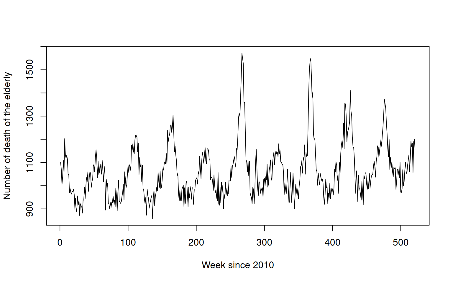
11.1.5 Importing from Excel
To import your Excel into R, first save your Excel file as a comma-separated (CSV) file by clicking on “File -> Save as” and select CSV.
Then, you can load this CSV-file into R using the command
11.1.6 Exercises: Exporting and Importing
See Section 18.0.30 for solutions.
Create a data frame with the columns x, y, and z, each containing 100 standard normal random numbers. Write this data frame to your working directory as “my_data_frame.txt”. Quit RStudio and use a text editor to add two additional entries (lines). Start RStudio again and import the modified data frame as d.
Open Calc (or Excel) and create a dummy file with some data. Find a way to import it into R using read.table(). (Hint: use the CSV format).
Load the population data on Swiss cities from (https://www.bfs.admin.ch/bfsstatic/dam/assets/12647632/appendix) into R and plot the population size of 1930 against that of 2018 for each city. Exclude the total population of Switzerland (first row).